Introduction
Congratulations on getting EVN data! What's next?
JIVE correlates all EVN observations and performs a preliminary reduction using the EVN pipeline. At this point you would have received an email from your EVN Support Scientist with details on how to access and download your data. You should take a look at the results from the pipeline analysis. In general the pipeline results are expected to be used only as a guide and should not be considered as a final science product. We recommend using the amplitude calibration table from the pipeline as the starting point of a manual calibration of the data. The fringe-fit, bandpass calibration, and imaging should thus be done by the user.
We recommend using AIPS to perform the initial reduction and calibration of EVN data as, to-date, other packages do not have the ability to fringe fit data, which is integral for non-connected element arrays.
Martin Shepherd's Difmap program can also be used for imaging and self-calibrating EVN data.
This page is intended to be a guide for new users that want to analyze EVN data, describing the standard steps that are performed during the data reduction. A basic knowledge of radio interferometric data and AIPS is required to fully understand all the steps.
Obtaining the data
EVN Data Archive
After correlation, the EVN Support Scientists will send you an email with details on how to access and download your data. The data, together with the EVN pipeline results, are stored at the EVN Data Archive, where you can find useful information concerning your experiment:
- Feedback page containing the feedback from each station and providing information about local circumstances during the observation.
- Logfiles page containing the station logfiles, schedule files, and all detailed instrumental settings during the observation.
- Standard plots showing the quality of the correlated experiment. These plots are produced after the correlation and show the behavior of the stations along the observation.
- Pipeline results providing a more detailed impression of the quality of the data. It contains plots for each source separately. Whereas the final results from the pipeline should not be considered for science results, we encourage the users to use the a-priori amplitude calibration table (CL2) and flag table (FG1) from the pipeline to start a manual calibration (see below).
- Fits files with the correlated data in IDI format.
Loading the data into AIPS
AIPS runs in a dedicated environment that do not support long path names. For this reason it is recommended to set up an environment variable, MYDIR, with the working directory where your data are:
We note that AIPS automatically recognizes PWD as an environment variable, thus in case that your working directory is the same as the directory from where AIPS is launched you do not need the previous step.
Now we can start AIPS by typing:
The tv=local:0 parameter is optional but it assures that a new graphical window will be open in case of having other AIPS sessions already opened.
AIPS will then ask you for a user number. This guide assumes you are using an "empty" AIPS user number (not used before or with no data inside).
Loading the data into AIPS using the task FITLD:
datain 'MYDIR:EXPERIMENT_1_1.IDI
digicor -1
doconcat 1
ncount n
outname 'name'
go fitld
Assuming that the used user number was empty, the data is now loaded into catalog number 1 (you can list all the catalog entries with pca).
AIPS output
The message server will notify you that your data are being loaded. This may take a while as a function of the size of your data. The data will have finished loading when the message server says that FITLD "Appears to have ended successfully."Now we need to load the file containing the calibration tables and copy the appropriate ones to our data:
datain 'MYDIR:EXPERIMENT_tasav.FITS
doconcat -1
ncount 1
outname 'name'
go fitld
AIPS output
Now you will found these data as a second catalog entry (can be selected with getn 2).We generally recommend using the a-priori amplitude calibration provided by the EVN pipeline (CL2 from this last file), and applying the flags from FG1 (which for example automatically flags the off-source times for each telescope). We can copy these tables to our data using TACOP:
getn 2
geton 1
inext 'CL'
inver 2
ncount 1
go tacop
inext 'FG'
inver 1
ncount 1
go tacop
AIPS output
The task TACOP copies the table CL number 2 (selected by invers) from the tasav file (getn 2) to our data (geton 1). We repeat the same but for the FG table 1.We can check that both tables have been correctly copied by typing getn 1 and imh, which shows us the header of that catalog entry. The output should be equivalent to:
AIPS output
AIPS 1: Image=MULTI     (UV)         Filename=EM121B      .UVDATA.   1
AIPS 1: Telescope=EVN                Receiver=VLBA
AIPS 1: Observer=EM121B              User #= 1212
AIPS 1: Observ. date=23-OCT-2016     Map date=31-MAR-2017
AIPS 1: # visibilities    679677     Sort order  TB
AIPS 1: Rand axes: UU-L-SIN  VV-L-SIN  WW-L-SIN  TIME1  SUBARRAY
AIPS 1:            FREQSEL  SOURCE  INTTIM  ANTENNA1  ANTENNA2  CORR-ID
AIPS 1: ----------------------------------------------------------------
AIPS 1: Type    Pixels   Coord value     at Pixel     Coord incr   Rotat
AIPS 1: COMPLEX      3   0.0000000E+00       1.00  1.0000000E+00    0.00
AIPS 1: STOKES       4  -1.0000000E+00       1.00 -1.0000000E+00    0.00
AIPS 1: FREQ        32   4.9269900E+09       1.00  5.0000000E+05    0.00
AIPS 1: IF           8   1.0000000E+00       1.00  1.0000000E+00    0.00
AIPS 1: RA           1    20 31 51.780       1.00       3600.000    0.00
AIPS 1: DEC          1    41 31 18.300       1.00       3600.000    0.00
AIPS 1: ----------------------------------------------------------------
AIPS 1: Coordinate equinox 2000.00
AIPS 1: Maximum version number of extension files of type HI is   1
AIPS 1: Maximum version number of extension files of type FG is   1
AIPS 1: Maximum version number of extension files of type AT is   1
AIPS 1: Maximum version number of extension files of type NX is   1
AIPS 1: Maximum version number of extension files of type CL is   2
AIPS 1: Maximum version number of extension files of type CT is   1
AIPS 1: Maximum version number of extension files of type FQ is   1
AIPS 1: Maximum version number of extension files of type AN is   1
AIPS 1: Maximum version number of extension files of type SU is   1
AIPS 1: Keyword = 'OLDRFQ  '  value =  4.92699000D+09
AIPS 1: Keyword = 'CORRELAT'  value = 'SFXC    '
Here AIPS shows us the basic data from our experiment. In particular, we can see:
- The number of recorded polarizations (STOKES 4, which means full polarization: RR, LL, RL, LR).
- The frequency setup of the observation (FREQ 32 4.9269900E+09 and IF 8, which means that we have observed at the central frequency of 4.9 GHz with 8 IFs, or subbands, of 32 channels each). Each channel with a bandwidth of 0.5 MHz.
- The coordinates of the phase center (RA and DEC).
- The existing tables in the data (e.g. 1 FG table and 2 CL tables). CL1 corresponds to the pristine calibration table and CL2 to the a-priori calibration table that we just copied from the pipeline, and contains the amplitude correction for each station and the parallactic angle corrections.
Inspecting the data
Before starting the calibration we should take a look at the data. We can start running LISTR and PRTAN to get information about the observed sources and the stations that participated during the observation.
getn 1
optype 'SCAN'
go listr
AIPS output
LISTR will show us the scans of the experiment, at which time they were observed and which source. Finally it will summarize all the observed sources and how many visibilities have been recorded per source, and the frequency set up (the central frequency, bandwidth and spectral separation for each IF).getn 1
go prtan
AIPS output
PRTAN reads the information available in the AN table (antenna information) and provides the frequency setup for each station (we note that in the EVN different stations can exhibit slightly different frequency setups due to different receivers/configurations). At the end it also shows a summary with all the stations that participated in the observation and their coordinates with respect to the Earth's center.One of the (many!) nice things about VLBI is that most terrestrial RFI will not correlate. The FG1 table that we already imported flags some data such as the edge-channels or the off-source times. Nonetheless, there are times that flagging is necessary. AIPS has several flagging tasks such as UVFLG, TVFLG, SPFLG and RFLAG. Use plotting tasks such as POSSM and UVPLT to determine if you wish to flag any data. You should also look at the pipeline plots (e.g., plots of amplitude and phase against frequency channel) as they will provide invaluable information about the location of bad data. It is recommended that obvious bad data is flagged from your calibrators to ensure a good calibration. See an example of the plots that you can produce with these tasks in the following buttons:
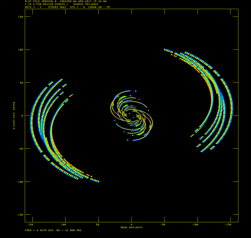
uv-coverage of an EVN observation. Produced with UVPLT using bparm 6 7 2 0.
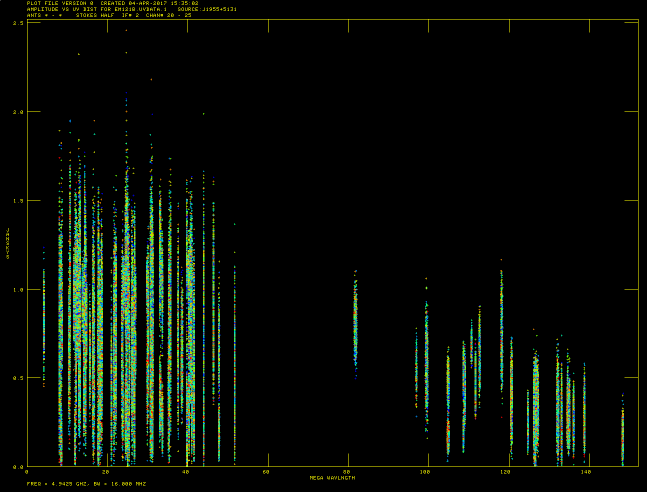
Amplitude versus uv-distance plot. Note that the source is slightly resolved at the longest distances (lower amplitudes). Produced with UVPLT using bparm 0.
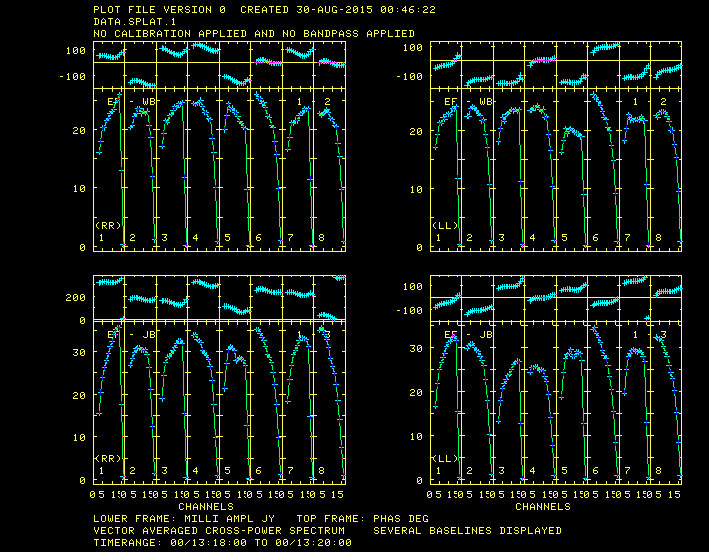
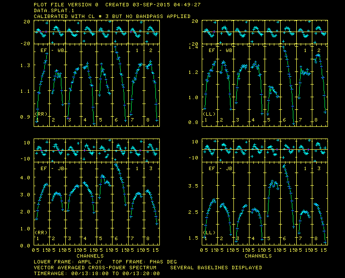
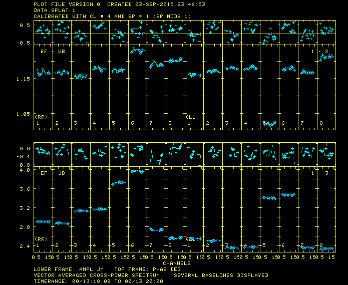
Plot of the amplitude and phase as a function of the frequency for different baselines and polarizations. Note the phase offset between IFs (due to instrumental delays), which will be corrected for with the first fringe-fit and the bandpass shape at each IF, which will be corrected with a bandpass calibration. Produced with POSSM.
Calibration
If your observation was conducted at frequencies ≲ 5 GHz you probably want to correct for ionospheric effects. Given that the stations are located at huge distances (up to 10,000 km apart), the ionospheric conditions can be really different at each location, affecting in a different way to each station.
Although there are different approaches to correct for the ionospheric effects, here we will show how to run VLBATECR, which is part of the VLBA utilities. First, we need to type (if we have not done it before) run vlbautil to load all these utilities. And then:
getn 1
go vlbatecr
This task will download the appropriate files from CDDIS and then it will run TECOR with these files. We will get a new CL table (CL3) containing these corrections. Note that in the following the user guide assumes that you did not perform this correction and the next calibration takes CL2. In case you correct for this effect, all gainu/gainv parameters will need to use one version higher than mentioned in theuUser guide (i.e. gainv 3 instead of gainv 2, and so on).
Removing instrumental delay
You may have noticed in POSSM that there is not only a gradient in phase within each IF, but the mean phases for each IF are also quite different with jumps in between. This is due to the independent signal paths for each IF, and must be corrected for (there are not physical jumps in the phases between IFs, they clearly have an instrumental origin).
In this step we will be correcting for instrumental delays, the phase jumps between IFs, and as such we only want data over a short time period because we do not want changes as a function of time to come into play (these delays should be constant along the whole observation). This is why it is important to have bright calibrators for VLBI observations! The effect of removing instrumental delays is to bring all the phases to zero, at least for the chosen time range. To correct the instrumental delay choose a few minutes on a bright fringe-finder (FF) when all antennas observed and the data is free of RFI.
getn 1
timerang d1 h1 m1 s1 d2 h2 m2 s2
docal 1
gainu 2
weightit 1
refant n
solint t
dparm(9) 1
cmethod 'dft'
snver 1
go fring
- timerange uses AIPS time syntax and it will select the data between d1/h1:m1:s1 and d2/h2:m2:s2.
- weightit 1 allows to modify the data weights. In the case of the EVN this is mandatory as we have significant differences between stations (e.g. we typically observe with stations with diameters ranging 20 to 100-m, producing a huge difference in sensitivity).
- refant n. You should chose as reference station one of the most sensitive and with highest-quality data in this scan.
- solint t sets the solution interval (in minutes, the default 0 means 10 min). The t value should be always larger than the time range to ensure we only get one data point.
- dparm(9) 1 tells AIPS to not fit the rates.
AIPS output
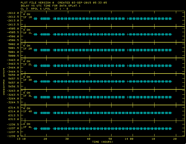
Make sure to look at the AIPS message server. It provides a feedback of the determined delays, phases, and rates and the signal-to-noise of the solutions. At the end AIPS shows how many solutions have been found and how many solutions have failed. Ideally there will be solutions for all IFs on all antennas.If you look now at the header of the file (with imh), you will notice that there is a new table: SN1. This table contains the solutions from this fringe-fit. You can use SNPLT to look at the delay solutions:
getn 1
inext 'sn'
invers 1
opty 'dela'
dotv 1
nplots 8
go snplt
The reference antenna should display a zero delay correction.
When you are happy with the SN table, you can apply it to your CL table (we will take CL2, apply the solutions in SN1 and it will create a CL3 table).
getn 1
gainver 2
gainuse 3
snver 1
interpol ''
opcode 'cali'
refant n
go clcal
We can look at the new calibration table with SNPLT (using inext 'cl') and POSSM again.
Each station has been corrected for instrumental delays using one solution per IF and polarization, which is extrapolated to the whole observation.
Amplitude and phase as a function of the frequency for different baselines and polarizations after correct for instrumental delays. Note that now the phases are centered on zero (they now exhibit a small scatter of few degrees).
We have considered here the most common case where we have a time range where all stations were observing without problems. However, this is not always true. We can have observations were only part of the stations were observing the fringe-finder in given scan, and the other stations were observing the fringe finder in a different scan (either the same source or a different one). This can happen, for example, in the case of observing with Asian, European, and American stations. At a particular time not all stations are available to observe.
- In this case, we will run FRING as mentioned before on the first scan.
- We run CLCAL in the same way, creating CL3 with only one change: optype 'CALP'. With this option SN1 will keep the data from the stations that were not available in that scan.
- Now, we run again FRING on the second timerange that includes the other stations. dofit a1, a2, ...; snver 2. Where a1, a2, ... are the stations that were not included previously. This makes that FRING only fits solutions for these stations, and not for the ones that have been already fit.
- Finally, we run CLCAL applying this new SN table to CL3, which will create CL4. This time with optype 'CALI'.
Frequency and time-dependent phase calibration
We have corrected for the instrumental delay. However, we now need to correct for delays and rates as a function of time, which will be done by fringe-fitting the data. Consequently we will be using a smaller solution interval.
getn 1
calsour 'sour1', 'sour2', ''
docal 1
gainu 3
timerang 0
weightit 1
refant n
solint t
aparm(5) 1
aparm(9) 1
dparm 1 200 50 i
search n2, n3, n4
snver 2
go fring
- aparm(5) 1 means that we will combine all IFs to improve the signal-to-noise ratio of the solutions.
- dparm sets the delay and rate windows within which to find solutions. i must be set equal to the integration time of the data (typically 1 or 2 s).
- search sets the second, third, and forth stations to be used as reference if refant fails.
- calsour sets the sources to be considered during the fringe-fitting. Basically we should consider the fringe-finders and all other calibrators that are strong enough.
- solint should be much smaller now as we want to correct for delays and rates. We can start with a value of 1 min (and increase if we do not get good solutions).
- aparm(6) 3 can be used to produce a more detailed output (optional).
AIPS output
The solutions have been written in SN2. You can look at the AIPS log and find information about the fit and how many solutions have been found/failed:LOCALH> FRING2: Fitted phases, rates, delays and SNR: [ P = phase(deg), LOCALH> FRING2: R = rate(mHz), D = Single-Band Delay(nsec), S = SNR ] LOCALH> FRING2: Ant(02): Phas= 19.6 rate= -0.70 delay= 0.05 SNR=2666.8 LOCALH> FRING2: Ant(03): Phas= -20.6 rate= -0.22 delay= 0.02 SNR=1886.7 LOCALH> FRING2: Ant(07): Phas= 29.0 rate= -0.01 delay= 0.03 SNR=2861.0 LOCALH> FRING2: Ant(08): Phas= -66.3 rate= -1.71 delay= 0.03 SNR=1680.1 LOCALH> FRING2: Standard RMS errors (deg, mHz, nsec): LOCALH> FRING2: Ant(02): Phas= 0.02 rate= 0.002 delay= 0.000 LOCALH> FRING2: Ant(03): Phas= 0.03 rate= 0.003 delay= 0.001 LOCALH> FRING2: Ant(07): Phas= 0.02 rate= 0.002 delay= 0.000 LOCALH> FRING2: Ant(08): Phas= 0.03 rate= 0.003 delay= 0.001 LOCALH> FRING2: Found 800 good solutions LOCALH> FRING2: Failed on 24 good solutions LOCALH> FRING2: Appears to have ended successfully
Now we can repeat the same steps that we conducted after the first FRING to look at the solutions (now recorded in SN2) with SNPLT.
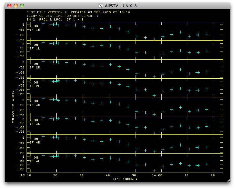
Solutions obtained in SN2 (delay as a function of the time in SNPLT with opty 'dela').
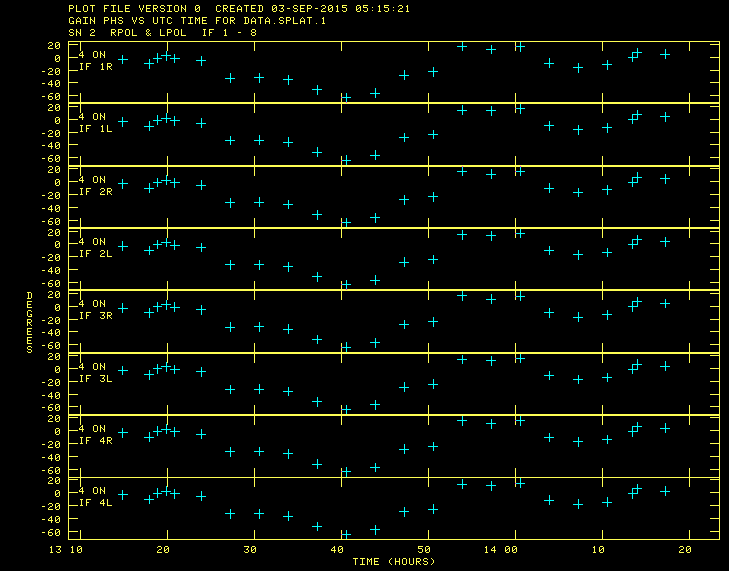
Solutions obtained in SN2 (phase as a function of the time in SNPLT with opty 'phas').
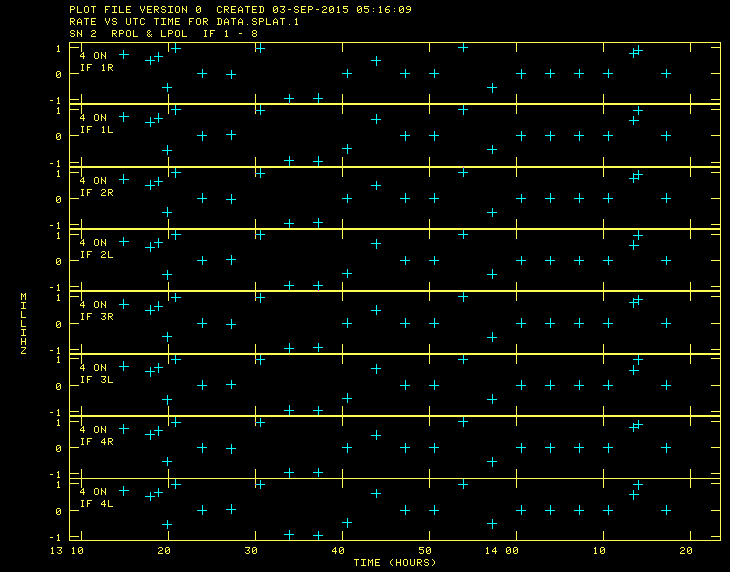
Solutions obtained in SN2 (rate as a function of the time in SNPLT with opty 'rate').
If the solutions look OK we can apply them to create a new calibration table (CL4). In this case, we will apply the solutions from each of the used calibrators to themselves, and finally the solutions from the phase calibrator will be also extrapolated to the target source (if we have conducted a phase-referencing observation).
getn 1
calsour 'calibrator-i', ''
sour calsour
doblank -1
dobtwe 1
docal 1
gainv 3
gainu 4
snver 2
refant n
interpol 'self'
opcode 'CALI'
go clcal
- calsour and sour should be the same and we should run multiple times CLCAL to apply the solutions for all the used calibrators.
- interpol must be 'self' as we are applying solutions from a particular calibrator to itself.
- opcode 'CALI' means that uncalibrated data will be flagged.
getn 1
calsour 'phase-calibrator', ''
sour calsour
docal 1
gainv 3
gainu 4
snver 2
refant n
interpol 'self'
opcode 'CALI'
go clcal
source 'target', ''
interpol 'ambg'
go clcal
We should look for possible bad times were the solutions were not properly obtained (e.g. the phases were rapping and coherence is completely lost). Those times would produce bad-quality data that should be manually removed in the final stages of the calibration.
If you have an image of the calibrator used in FRING, with an AIPS catalogue entry i (i.e. you select it with getn i), you can run FRING with the following additional paramenter:
get2n i
which selects that image to be used as a model of the source during the fringe-fitting.
For example, you can do a first calibration of your data, obtain an accurate image of your calibrator, and then repeat again the whole calibration using this image as a model in the FRING.
In this case we should also set cmethod 'DFT' to improve the fringe-fitting.
Bandpass calibration
Finally, we need to correct for the response of the receiver as a function of frequency. This is done via a bandpass calibration using BPASS.
getn 1
calsour 'bandpass-calibrator', ''
docal 1
refant n
solint -1
weightit 1
cmethod 'dft'
soltype 'l1r'
bpassprm(1) 0
bpassprm(2) 1
bpassprm(10) 1
go bpass
We can now look at the solutions again with POSSM, for example setting aparm 0, 1, 0, 2, -180, 180, 0, 2, 3 to show both amplitude and phase at the same time.
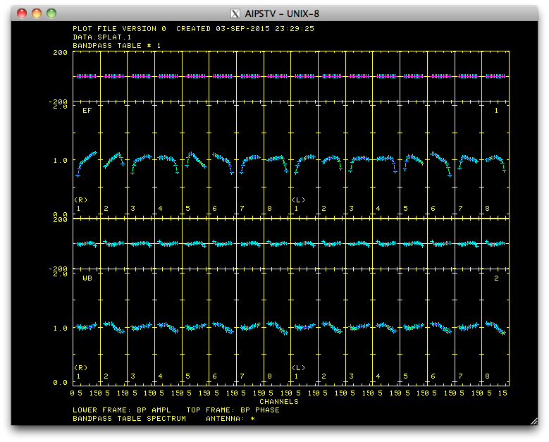
Solutions from the bandpass calibration (BP1 table).
Amplitudes and phases as a function of the frequency after applying CL4 and BP1. Note how now both amplitudes and phases are consistent along the full bandwidth with small deviations.
Split and storage the data
We are now ready to apply our calibration tables to the data. We will split the data to make imaging easier (e.g. creating different data sets for each source), and in the process of splitting the data we will apply CL4, BP1 and all FG tables to these data.
getn 1
source ''
docal 1
gainu 4
doband 1
bpver 1
flagv 0
aparm 2 1 0
go split
If you check now the available catalogue entries in our session (with pcat) you will see that there is a SPLIT file for each source, containing the calibrated data.
If you wish to store these files outside AIPS, in FITS format, you can run FITTP:
getn n
dataout 'MYDIR:filename.uvfits'
go fittp
AIPS output
You will now find a new file in the MYDIR directory containing the calibrated data for the selected source. Repeat this process with all files you want to store. Note that AIPS is case-insensitive, and thus all the created files will exhibit capital letters.Initial imaging with AIPS
Cleaning and imaging
As mentioned in the introduction, the imaging process can be done either in AIPS or in Difmap. Here we show a basic running of the AIPS imaging and how to obtain a map of your source. See the end of this page to find a more detailed tutorial on how to image and self-calibrate your data within Difmap and AIPS in case of phase-referencing experiments, or how to analyze EVN spectral line data.
The AIPS task to image your data is IMAGR.
getn n
source ''
imsize 512
cellsize x
niter 10000
gain 0.05
cmethod 'dft'
robust 0
dotv 1
go split
AIPS output
You will find two new files: an IBM001 file and an ICL001. The first one represents the image of your synthesized beam. The second one is the cleaned image of your source.You can look at your images by selecting the file with getn i and tvall. You can change interactively the colorscale and contrast with the mouse and keys. Run tvps to switch between colorscales or grayscales.
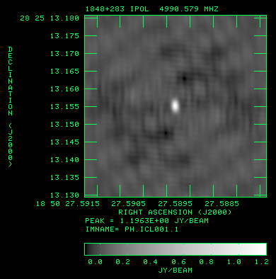
Clean image after running IMAGR.
Statistics from your image
There are two basic tasks in AIPS to perform measurements in your image, imstat (or tvstat) and jmfit.
imstat
imstat tells you the statistics of the image. After showing your image with tvall you just need to run imstat. You will see a message log as the following, reporting the mean, rms, maximum, minimum and minimum brightness and their positions in the image.
AIPS output
AIPS 2: Mean= 7.078E-04 rms= 5.194E-02 JY/BEAM  over     1048576. pixels
AIPS 2: Maximum= 1.5677E+00 at    512    513     1    1    1    1    1
AIPS 2: Skypos: RA 05 55 30.80561200  DEC 39 48 49.1649800
AIPS 2: Skypos: IPOL  4867.125 MHz
AIPS 2: Minimum=-1.9778E-01 at    121   1020     1    1    1    1    1
AIPS 2: Skypos: RA 05 55 30.80900551  DEC 39 48 49.2156799
AIPS 2: Skypos: IPOL  4867.125 MHz
AIPS 2: Flux density =  5.1963E+00 Jy   Beam area = 142.82 pixels
tvstat
tvstat is analog to imstat but you are able to select a particular region of the image where to perform the statistics. This can be useful to measure the rms of the image (selecting a large region around your source but without including it), and the flux density of your source. Once you run tvstat you are able to set the region graphically with the mouse.
jmfit
jmfit fits a gaussian to your image. The recommended way to run it is with tvall; tvwin; go jmfit, which shows you the image (tvall), allows you to select a region of the image around your source (tvwin), and run the gaussian fit (jmfit). This last command writes the solution in the message log:
AIPS output
LOCALH> JMFIT2: ********* Solution from JMFIT *********************************
LOCALH> JMFIT2:
LOCALH> JMFIT2: Component   1-Gaussian
LOCALH> JMFIT2:   Peak intensity    = 1.5311E+00 +/- 4.93E-02 JY/BEAM   ( 31.05)
LOCALH> JMFIT2:   Integral intensity= 1.7172E+00 +/- 9.23E-02 JANSKYS
LOCALH> JMFIT2:   X-position        =    512.138 +/-   0.2548 pixels
LOCALH> JMFIT2:   Y-position        =    513.182 +/-   0.1116 pixels
LOCALH> JMFIT2:                       RA 05 55 30.80561080 +/-  0.000002211
LOCALH> JMFIT2:                       DEC 39 48 49.1649981 +/-   0.00001116
LOCALH> JMFIT2:   Major axis        =  18.914 +/-  0.6092 pixels
LOCALH> JMFIT2:   Minor axis        =   7.474 +/-  0.2407 pixels
LOCALH> JMFIT2:   Position angle    = 100.857 +/-  1.222 degrees
LOCALH> JMFIT2:   Major axis        = 0.0018914 +/- 0.0000609 asec
LOCALH> JMFIT2:   Minor axis        = 0.0007474 +/- 0.0000241 asec
LOCALH> JMFIT2:   Position angle    = 100.857 +/-  1.222 degrees
LOCALH> JMFIT2:   RASHIFT=  -0.000014 DECSHIFT=   0.000018 to center on pixel
LOCALH> JMFIT2:   - - - - - - - - - - - - - - - - - - - - - - - - - - - - - -
LOCALH> JMFIT2:                   Deconvolution of component in pixels
LOCALH> JMFIT2:                        Nominal     minimum     maximum
LOCALH> JMFIT2:     Major ax             4.810       0.000       5.845
LOCALH> JMFIT2:     Minor ax             0.000       0.000       7.051
LOCALH> JMFIT2:     Pos ang             65.386      41.485     102.263
LOCALH> JMFIT2:                   Deconvolution of component in asec
LOCALH> JMFIT2:                        Nominal     minimum     maximum
LOCALH> JMFIT2:     Major ax          0.000481    0.000000    0.000584
LOCALH> JMFIT2:     Minor ax          0.000000    0.000000    0.000705
LOCALH> JMFIT2:     Pos ang          65.386246   41.485229  102.263382
LOCALH> JMFIT2:   Component may be unresolved or resolved, use caution
LOCALH> JMFIT2:   - - - - - - - - - - - - - - - - - - - - - - - - - - - - - -
LOCALH> JMFIT2: returns adverbs to AIPS
LOCALH> JMFIT2: Appears to have ended successfully
Further steps
We have shown the basics steps to analyze EVN data. But further steps can be done to improve the results and/or specific actions must be done as a function of what kind of observation you are analyzing.
In the following you can select the chapters that best suit for your data.